As you will recall, the statement of the problem is as follows:
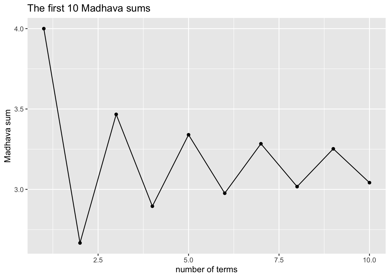
Recall the function madhavaPI() from Section 3.4.1. Use this function to write a function called madhavaGraph() that will do the following: given a number \(n\), the function uses ggplot2 to produce a line graph of the first \(n\) approximations to \(\pi\) using the initial terms of the Madhava series.
The plot should be a line graph similar to the one produced by the collatz() functions from this Chapter. The function should take a single argument n, whose default value is 10.
It should validate the input: if the number entered is not at least 1, then the function should should explain to the user that the he/she must enter a positive number, and then stop.
Outline
Based on the specification in the problem, you can set up an initial outline of the desired function, as follows:
madhavaGraph <- function(n = 10) {

  validate the input: if n isn't at least 1, stop the function

  find the sums:
    * the sum of the first term (4)
    * the sum of the first and second terms (4 - 4/3)
    * the sum of the first three terms ( 4 - 4/3 + 4/5)
    * and so on until ...
    * the sum of the first n terms
  make sure these sums are stored in a vector (let's call it "results")

  make the plot:
    - the vector 1:n (call it "terms") gives the x-coordinates of the points
    - the results vector gives y-coordinates

}
As you can see, the body of the function has three primary parts:
validating the input
finding the sums and storing them in the results vector
making the plot.
I’ll leave Part 1 entirely to you, but say a bit more about parts 2 and 3.
Making the Graph
First we’ll think about the graph. Since it is made from functions in the ggplot2 package, you will need to make sure that you load the package when you are designing the function.The function itself does not load ggplot2, so you should make sure to tell anyone who plans to use the function to load it!
library(ggplot2)
Now suppose that the value of the parameter n is 10. Then by the time you get around to making the graph you’ll have the terms:
terms <- 1:n
terms
## [1] 1 2 3 4 5 6 7 8 9 10
You’ll also have the sums, another vector of length 10:
From our study of the Collatz function, we know that the way to make a line graph of these points is:
plotTitle <- paste0("The first ", n, " Madhava sums")
  p <- ggplot(mapping = aes(x = terms, y = results)) +
    geom_point() + geom_line() +
    labs( x = "number of terms", y = "Madhava sum",
          title = plotTitle)
  print(p)
Hence we can fill in the outline of our function a bit:
madhavaGraph <- function(n = 10) {

  validate the input: if n isn't at least 1, stop the function

  find the sums:
    * the sum of the first term (4)
    * the sum of the first and second terms (4 - 4/3)
    * the sum of the first three terms ( 4 - 4/3 + 4/5)
    * and so on until ...
    * the sum of the first n terms
  make sure these sums are stored in a vector (let's call it "results")

 plotTitle <- paste0("The first ", n, " Madhava sums")
  p <- ggplot(mapping = aes(x = terms, y = results)) +
    geom_point() + geom_line() +
    labs( x = "number of terms", y = "Madhava sum",
          title = plotTitle)
  print(p)

}
Finding and Storing the Sums
The outline for this part of the task looked like:
get the sum of the first term (just 1)
get the sum of the first and second terms (\(4 - 4/3\))
get the sum of the first three terms (\(4 - 4/3 + 4/5\))
and so on until …
get the sum of the first n terms
At each step in above process, we will need to store our sum in the results vector, so that it isn’t lost.
The natural way to accomplish the above task is to use a for-loop in which we iterate by index and store results. The outline of such a loop is:
results <- numeric(n)
for ( i in 1:n ) {

  results[i] <- the sum of the first i terms

}
We already know how to find the sum of the first \(i\) terms: we can just use the function madhavaPI() from Chapter 3:
madhavaPI <- function(n = 1000000) {
  k <- 1:n
  terms <- (-1)^(k+1)*4/(2*k-1)
  sum(terms)
}
Hence when you are working inside the loop, you can get and store the results all in one line:
results[i] <- madhavaPI(i)
Well, to be totally truthful, you can do this provided that R knows what madhavaPI() is. Hence you must either:
hope that whoever uses madhavaGraph() has madhavaPI() in their Global Environment so that madhavaGraph() can look up the name madhavaPI when it needs it, or
define madhavaPI() inside the body of madhavaGraph(), before you start computing any sums.
The latter seems to be the safer choice!
Put It All Together
You still have the task of filling in the outline completely and then testing madhavaGraph() until it works.